43 format data labels pane excel
How to Print Labels From Excel? | Steps to Print Labels ... Navigate towards the folder where the excel file is stored in the Select Data Source pop-up window. Select the file in which the labels are stored and click Open. A new pop up box named Confirm Data Source will appear. Click on OK to let the system know that you want to use the data source. Again a pop-up window named Select Table will appear. Format elements of a chart - support.microsoft.com Right-click the chart axis, and click Format Axis. In the Format Axis task pane, make the changes you want. You can move or resize the task pane to make working with it easier. Click the chevron in the upper right. Select Move and then drag the pane to a new location. Select Size and drag the edge of the pane to resize it.
How to Print Labels from Excel - Lifewire Select Mailings > Write & Insert Fields > Update Labels . Once you have the Excel spreadsheet and the Word document set up, you can merge the information and print your labels. Click Finish & Merge in the Finish group on the Mailings tab. Click Edit Individual Documents to preview how your printed labels will appear. Select All > OK .
Format data labels pane excel
Prepare your Excel data source for a Word mail merge In your Excel data source that you'll use for a mailing list in a Word mail merge, make sure you format columns of numeric data correctly. Format a column with numbers, for example, to match a specific category such as currency. If you choose percentage as a category, be aware that the percentage format will multiply the cell value by 100. Pie of Pie Chart in Excel - Inserting, Customizing - Excel ... This is going to open a Format Data Labels pane at the right of excel. Mark the percentage, category name, and legend key. Select the position of data labels at Outside End. Select the fill color for data labels as white as we will change the chart background in the coming section. You can do it from the fill tab of the opened pane. Format Chart Axis in Excel – Axis Options Dec 14, 2021 · Axis Options : Number Format. We can change the format of axis values of the chart in excel in the same way we do for the cell entries. Below are the number formats available for chart values in excel. It is currently set to general number format. We would choose the currency from the list.
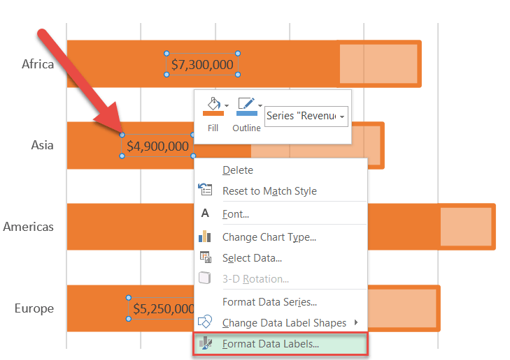
Format data labels pane excel. How do you format data series in Excel? To format data labels in EÎl , choose the set of data labels to format . To do this, click the " Format " tab within the "Chart Tools" contextual tab in the Ribbon. Then select the data labels to format from the "Chart Elements" drop-down in the "Current Selection" button group. How do I show the Format Data Series pane in Excel? Formatting data labels and printing pie charts on Excel ... 2. When formatting data labels on an extended bar of pie chart: Excel does not allow me to: i format all the data labels at once to show 3 elements: category name, value and percentage. In the label options, I can tick these 3 elements, but chart wont show them. I have to go in and edit each data label in turn. As there are 48, this is not ... Excel Charts - Aesthetic Data Labels - Tutorialspoint Step 1 − In the Format Data Labels pane, click the Label Options icon. Step 2 − Under Data Label Series, click Clone Current Label. This will enable you to apply your custom data label formatting quickly to the other data points in the series. Data Labels with Effects. You can opt for many things to change the look and feel of the data ... Change the format of data labels in a chart To get there, after adding your data labels, select the data label to format, and then click Chart Elements > Data Labels > More Options. To go to the appropriate area, click one of the four icons ( Fill & Line , Effects , Size & Properties ( Layout & Properties in Outlook or Word), or Label Options ) shown here.
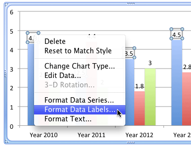
Format Data Label: Label Position - Microsoft Community when you add labels with the + button next to the chart, you can set the label position. In a stacked column chart the options look like this: For a clustered column chart, there is an additional option for "Outside End" When you select the labels and open the formatting pane, the label position is in the series format section. Does that help? How to Customize Your Excel Pivot Chart Data Labels - dummies Excel displays the Format Data Labels pane. Check the box that corresponds to the bit of pivot table or Excel table information that you want to use as the label. For example, if you want to label data markers with a pivot table chart using data series names, select the Series Name check box. How to hide zero data labels in chart in Excel? If you want to hide zero data labels in chart, please do as follow: 1. Right click at one of the data labels, and select Format Data Labels from the context menu. See screenshot: 2. In the Format Data Labels dialog, Click Number in left pane, then select Custom from the Category list box, and type #"" into the Format Code text box, and click Add button to add it to Type list box. Edit titles or data labels in a chart - support.microsoft.com The first click selects the data labels for the whole data series, and the second click selects the individual data label. Right-click the data label, and then click Format Data Label or Format Data Labels. Click Label Options if it's not selected, and then select the Reset Label Text check box. Top of Page
How to change chart axis labels' font color and size in Excel? 1. Right click the axis where you will change all negative labels' font color, and select the Format Axis from the right-clicking menu. 2. Do one of below processes based on your Microsoft Excel version: (1) In Excel 2013's Format Axis pane, expand the Number group on the Axis Options tab, click the Category box and select Number from drop down ... Format Data Labels in Excel- Instructions - TeachUcomp, Inc. Nov 14, 2019 · Alternatively, you can right-click the desired set of data labels to format within the chart. Then select the “Format Data Labels…” command from the pop-up menu that appears to format data labels in Excel. Using either method then displays the “Format Data Labels” task pane at the right side of the screen. Format Data Labels in Excel ... Pie Chart in Excel - Inserting, Formatting, Filters, Data ... Click on Format Data Labels option. Consequently, this will open up the Format Data Labels pane on the right of the excel worksheet. Mark the Category Name, Percentage and Legend Key. Also mark the labels position at Outside End. This is how the chark looks. How to format axis labels as thousands/millions in Excel? Right click at the axis you want to format its labels as thousands/millions, select Format Axisin the context menu. 2. In the Format Axisdialog/pane, click Number tab, then in theCategorylist box, select Custom, and type[>999999] #,,"M";#,"K"into Format Codetext box, and click Addbutton to add it toTypelist. See screenshot: 3.
SQL Workbench/J User's Manual SQLWorkbench
2/ Right-click i.e. on the 1st histo. bar (A) > Add Data Labels (numbers are displayed a the top of the bars) 3/ Click one of the numbers that just displayed (the Format Data Labels pane opens on the right) > Check option "Value From Cells" > Select range C2:C7 > OK > Uncheck option "Value" demo.png (18.5 KiB) · 3

How to add total labels to stacked column chart in Excel?
How to add data labels from different column in an Excel chart? In the Format Data Labels pane, under Label Options tab, check the Value From Cells option, select the specified column in the popping out dialog, and click the OK button. Now the cell values are added before original data labels in bulk. 4. Go ahead to untick the Y Value option (under the Label Options tab) in the Format Data Labels pane.
How to Create Progress Charts (Bar and Circle) in Excel - Automate Excel
Add a DATA LABEL to ONE POINT on a chart in Excel | Excel ... You can now configure the label as required — select the content of the label (e.g. series name, category name, value, leader line), the position (right, left, above, below) in the Format Data Label pane/dialog box. To format the font, color and size of the label, now right-click on the label and select 'Font'. Note: in step 5. above, if ...

Format Data Label Options for Charts in PowerPoint 2013 for Windows
How to stagger axis labels in Excel 15. Next, right-click the Series "+ label" Data Labels and then, on the shortcut menu, click Format Data Labels. 16. In the Format Data Labels pane, with Label Options selected, set the Label Position to Below. 17. Under Label Contains, click on Value Form Cells. In the Data Label Range dialog box set the Select Data Label Range to refer

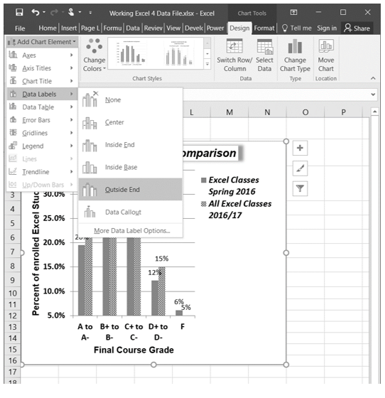
Common Tasks: Chart | Intro | Jan's Working with Numbers
Using Graphics to Represent Data Series (Microsoft Excel) Choose Format Data Series from the Context menu. Excel displays the Format Data Series task pane at the right side of the chart. In the task pane click the Fill & Line icon; it looks like a spilling paint bucket. Expand the Fill options by clicking the small triangle next to the Fill heading. (See Figure 2.) Figure 2. The Fill options of the ...

Excel 2013 Tutorial Formatting Data Labels Microsoft Training Lesson 28.6 - YouTube
Format Data Labels Task Pane Excel In the Chart Layouts group, select Add Chart Element > Data Labels > More Data Label Options This activates the Format Data Labels task pane. Under Label Contains, tick the check box Value From Cells. A dialog will pop up to let you specify the range to use. › Verified 3 days ago › Url: answers.microsoft.com Go Now

Format Data Label Options for Charts in PowerPoint 2013 for Windows
Excel tutorial: How to use data labels When first enabled, data labels will show only values, but the Label Options area in the format task pane offers many other settings. You can set data labels to show the category name, the series name, and even values from cells. In this case for example, I can display comments from column E using the "value from cells" option.

How to add labels to the mosaic plot - Microsoft Excel 2016
Format a Map Chart - support.microsoft.com Select the data point of interest in the chart legend or on the chart itself, and in the Ribbon > Chart Tools > Format, change the Shape Fill, or change it from the Format Object Task Pane > Format Data Point > Fill dialog, and select from the Color Pallette: Other chart formatting

Format Data Labels in Excel- Instructions - TeachUcomp, Inc.
Make Chart X Axis Labels Display below Negative Data - Excel How Aug 21, 2018 · #2 right click on the selected X Axis, and select Format Axis… from the pop-up menu list. The Format Axis pane will be displayed in the right of excel window. #3 on Format Axis pane, expand the Labels section, select Low option from the Label Position drop-down list box. Close the Format Axis pane.

31 Label Format In Excel - Labels Database 2020
Excel 2016 Tutorial Formatting Data Labels Microsoft ... FREE Course! Click: about Formatting Data Labels in Microsoft Excel at . A clip from Mastering Excel M...
Format Data Label Options in PowerPoint 2011 for Mac
Add or remove data labels in a chart Right-click the data series or data label to display more data for, and then click Format Data Labels. Click Label Options and under Label Contains , select the Values From Cells checkbox. When the Data Label Range dialog box appears, go back to the spreadsheet and select the range for which you want the cell values to display as data labels.

Excel 3-D Pie Charts
Excel tutorial: The Format Task pane You can also select a chart element first, then use the keyboard shortcut Control + 1. For example, if I select the data bars in this chart, then type Control + 1, the Format Task Pane will open with with the data series options selected. The Format Task pane stays open until you manually close the window.

Excel 2016 charts: How to use the new Pareto, Histogram, and Waterfall formats | PCWorld
Format Chart Axis in Excel – Axis Options Dec 14, 2021 · Axis Options : Number Format. We can change the format of axis values of the chart in excel in the same way we do for the cell entries. Below are the number formats available for chart values in excel. It is currently set to general number format. We would choose the currency from the list.
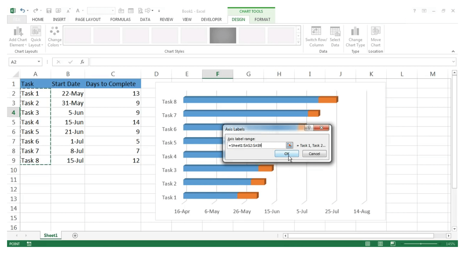
How to Make Gantt Chart in Excel? | Gantt Chart Excel - Zoho Projects
Pie of Pie Chart in Excel - Inserting, Customizing - Excel ... This is going to open a Format Data Labels pane at the right of excel. Mark the percentage, category name, and legend key. Select the position of data labels at Outside End. Select the fill color for data labels as white as we will change the chart background in the coming section. You can do it from the fill tab of the opened pane.
4.2 Formatting Charts – Beginning Excel
Prepare your Excel data source for a Word mail merge In your Excel data source that you'll use for a mailing list in a Word mail merge, make sure you format columns of numeric data correctly. Format a column with numbers, for example, to match a specific category such as currency. If you choose percentage as a category, be aware that the percentage format will multiply the cell value by 100.
Post a Comment for "43 format data labels pane excel"