39 how to add percentage data labels in excel bar chart

adding extra data labels - Excel Help Forum Re: adding extra data labels. No time to look at your file right now, so here's the quickie. create the data in the table that shows the actual numbers, not the %. add this data into the chart as a new series. change the series type to be a line chart. format the series to be on the secondary axis. format the series to show the data labels. Stacked bar charts showing percentages (excel) - Microsoft Community When you add data labels, Excel will add the numbers as data labels. You then have to manually change each label and set a link to the respective % cell in the percentage data range. Pls have a look at the second image below - In that image I have manually changed the data labels for 'Cat1'. Manually change the data label reference is easy.

Excel tutorial: How to build a 100% stacked chart with percentages F4 three times will do the job. Now when I copy the formula throughout the table, we get the percentages we need. To add these to the chart, I need select the data labels for each series one at a time, then switch to "value from cells" under label options. Now we have a 100% stacked chart that shows the percentage breakdown in each column.

How to add percentage data labels in excel bar chart

How to Add Percentages to Excel Bar Chart Once we do this we will click on our created Chart, then go to Chart Design >> Add Chart Element >> Data Labels >> Inside Base: Our chart will look like this: To lose the colors that we have on points percentage and to lose it in the title we will simply click anywhere on the small orange bars and then go to Format >> Shape Styles >> Shape Fill ... How to Create a Bar Chart With Labels Above Bars in Excel In the Format Data Labels pane, under Label Options selected, set the Label Position to Inside End. 16. Next, while the labels are still selected, click on Text Options, and then click on the Textbox icon. 17. Uncheck the Wrap text in shape option and set all the Margins to zero. The chart should look like this: 18. Add or remove data labels in a chart - support.microsoft.com Depending on what you want to highlight on a chart, you can add labels to one series, all the series (the whole chart), or one data point. Add data labels. You can add data labels to show the data point values from the Excel sheet in the chart. This step applies to Word for Mac only: On the View menu, click Print Layout.

How to add percentage data labels in excel bar chart. Count and Percentage in a Column Chart - ListenData Download the workbook. Steps to show Values and Percentage. 1. Select values placed in range B3:C6 and Insert a 2D Clustered Column Chart (Go to Insert Tab >> Column >> 2D Clustered Column Chart). See the image below. Insert 2D Clustered Column Chart. 2. In cell E3, type =C3*1.15 and paste the formula down till E6. How to Add Percentage Axis to Chart in Excel To do this, we will select the whole table again, and then go to Insert >> Charts >> 2-D Columns: To show percentages on a second axis, we first need to click anywhere on the orange bars that we have on our graph (this is not easy in this example as they are rather small). Once we do, we will right-click on it, and then select Format Data Series: How to Add Percentage Increase/Decrease Numbers to a Graph Trendline 1. It won't allow me to directly insert a date into the graph. If I insert a date outside the graph and attempt to move it into the desired position, then it seemingly goes behind the graph and is invisible. 2. "For the percentage increase/decrease to be used as data labels." Actual vs Budget or Target Chart in Excel - Variance on ... Aug 19, 2013 · Great question on how to add the percentage variance to the data labels. If you are using Excel 2013 there is a new feature that allows you to display data labels based on a range of cells that you select. It is the “Value From Cells” option in the Label Options menu.

Add or remove data labels in a chart - support.microsoft.com Tip: You can use either method to enter percentages — manually if you know what they are, or by linking to percentages on the worksheet.Percentages are not calculated in the chart, but you can calculate percentages on the worksheet by using the equation amount / total = percentage.For example, if you calculate 10 / 100 = 0.1, and then format 0.1 as a percentage, the number will … How to create a chart with both percentage and value in Excel? Create a chart with both percentage and value in Excel. To solve this task in Excel, please do with the following step by step: 1. Select the data range that you want to create a chart but exclude the percentage column, and then click Insert > Insert Column or Bar Chart > 2-D Clustered Column Chart, see screenshot: 2. How to show data label in "percentage" instead of - Microsoft Community If so, right click one of the sections of the bars (should select that color across bar chart) Select Format Data Labels. Select Number in the left column. Select Percentage in the popup options. In the Format code field set the number of decimal places required and click Add. (Or if the table data in in percentage format then you can select ... How to Use Excel to Make a Percentage Bar Graph - Techwalla Percentage bar graphs compare the percentage that each item contributes to an entire category. Rather than showing the data as clusters of individual bars, percentage bar graphs show a single bar with each measured item represented by a different color. Each bar on the category axis (often called the x-axis) represents 100 percent.

Understanding Excel Chart Data Series, Data Points, and Data Labels 19-09-2020 · Numeric Values: Taken from individual data points in the worksheet.; Series Names: Identifies the columns or rows of chart data in the worksheet. Series names are commonly used for column charts, bar charts, and line graphs. Category Names: Identifies the individual data points in a single series of data.These are commonly used for pie charts. Add Value Label to Pivot Chart Displayed as Percentage Aug 28, 2014. #1. I have created a pivot chart that "Shows Values As" % of Row Total. This chart displays items that are On-Time vs. items that are Late per month. The chart is a 100% stacked bar. I would like to add data labels for the actual value. Example: If the chart displays 25% late and 75% on-time, I would like to display the values ... Make a Percentage Graph in Excel or Google Sheets Creating a Stacked Bar Graph. Highlight the data; Click Insert; Select Graphs; Click Stacked Bar Graph; Add Items Total. Create a SUM Formula for each of the items to understand the total for each.. Find Percentages. Duplicate the table and create a percentage of total item for each using the formula below (Note: use $ to lock the column reference before copying + pasting the formula across ... Quickly create a positive negative bar chart in Excel Now create the positive negative bar chart based on the data. 1. Select a blank cell, and click Insert > Insert Column or Bar Chart > Clustered Bar. 2. Right click at the blank chart, in the context menu, choose Select Data. 3. In the Select Data Source dialog, click Add button to open the Edit Series dialog.

How-to Put Percentage Labels on Top of a Stacked Column Chart - Excel Dashboard Templates

How can I show percentage change in a clustered bar chart? Double-click it to open the "Format Data Labels" window. Now select "Value From Cells" (see picture below; made on a Mac, but similar on PC). Then point the range to the list of percentages. If you want to have both the value and the percent change in the label, select both Value From Cells and Values. This will create a label like: -12% 1.729.711

Quickly create a positive negative bar chart in Excel

Actual vs Budget or Target Chart in Excel - Variance on Clustered ... 19-08-2013 · Great question on how to add the percentage variance to the data labels. If you are using Excel 2013 there is a new feature that allows you to display data labels based on a range of cells that you select. It is the “Value From Cells” option in the Label Options menu.

How to Make Your Excel Bar Chart Look Better – MBA Excel

Add vertical line to Excel chart: scatter plot, bar and line ... May 15, 2019 · Add vertical line to Excel scatter chart; Insert vertical line in Excel bar chart; Add vertical line to line chart; How to add vertical line to scatter plot. To highlight an important data point in a scatter chart and clearly define its position on the x-axis (or both x and y axes), you can create a vertical line for that specific data point ...

33 How To Label Bar Graph In Excel

Create Dynamic Chart Data Labels with Slicers - Excel Campus 10-02-2016 · Typically a chart will display data labels based on the underlying source data for the chart. In Excel 2013 a new feature called “Value from Cells” was introduced. This feature allows us to specify the a range that we want to use for the labels. Since our data labels will change between a currency ($) and percentage (%) formats, we need a ...

Excel Dashboard Templates Friday Challenge Answer - Create a Percentage (%) and Value Label ...

How to Create a Timeline Chart in Excel - Automate Excel In order to polish up the timeline chart, you can now add another set of data labels to track the progress made on each task at hand. Right-click on any of the columns representing Series “Hours Spent” and select “Add Data Labels.” Once there, right-click on any of the data labels and open the Format Data Labels task pane.

Create Pie of Pie or Bar of Pie Charts in Excel - Free Excel Tutorial

Create Dynamic Chart Data Labels with Slicers - Excel Campus Feb 10, 2016 · This is because Excel 2010 does not contain the Value from Cells feature. Jon Peltier has a great article with some workarounds for applying custom data labels. This includes using the XY Chart Labeler Add-in, which is a free download for Windows or Mac. Step 6: Setup the Pivot Table and Slicer. The final step is to make the data labels ...

How to make a histogram in Excel 2019, 2016, 2013 and 2010

charts - Showing percentages above bars on Excel column graph - Stack ... 0. The easy answer is you can edit the pivot table: -Right-click on the column showing series and goto pivot table options. -Click on Show values as an option. -Click on the percentage of grand total. -Enjoy :) Note: Although it will change the original values also to percentage.

Art of Charts: Bubble grid charts: an alternative to stacked bar/column charts with lots of data ...

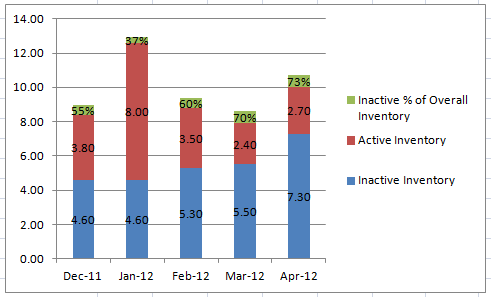
How to Add Total Data Labels to the Excel Stacked Bar Chart For stacked bar charts, Excel 2010 allows you to add data labels only to the individual components of the stacked bar chart. The basic chart function does not allow you to add a total data label that accounts for the sum of the individual components. Fortunately, creating these labels manually is a fairly simply process.

Share :