45 labels and values in excel
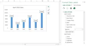
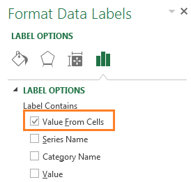
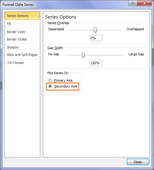
How to Find, Highlight, and Label a Data Point in Excel Scatter Plot? By default, the data labels are the y-coordinates. Step 3: Right-click on any of the data labels. A drop-down appears. Click on the Format Data Labels… option. Step 4: Format Data Labels dialogue box appears. Under the Label Options, check the box Value from Cells . Step 5: Data Label Range dialogue-box appears. How to Add Total Values to Stacked Bar Chart in Excel Step 4: Add Total Values. Next, right click on the yellow line and click Add Data Labels. Next, double click on any of the labels. In the new panel that appears, check the button next to Above for the Label Position: Next, double click on the yellow line in the chart. In the new panel that appears, check the button next to No line:
How to Count Unique Values in Excel - groovyPost To do this, select the cells containing your values in your spreadsheet. With the cells selected, take a look at the bottom of your Excel window (below the sheet labels). You'll see different...
Labels and values in excel
How to Add Axis Labels in Microsoft Excel - Appuals.com If you want to label the depth (series) axis (the z axis) of a chart, simply click on Depth Axis Title and then click on the option that you want. In the Axis Title text box that appears within the chart, type the label you want the selected axis to have. Pressing Enter within the Axis Title text box starts a new line within the text box. How to Edit Pie Chart in Excel (All Possible Modifications) As a result, there will be a new ribbon named Format Data Labels at the right side of your Excel file. Now, go to the Label Options menu >> Label Options group >> put a tick mark on the Percentage option. As a result, there will be percentage values too at the data labels. The result sheet would look like this. 👇 9. Custom Chart Data Labels In Excel With Formulas - How To Excel At Excel Follow the steps below to create the custom data labels. Select the chart label you want to change. In the formula-bar hit = (equals), select the cell reference containing your chart label's data. In this case, the first label is in cell E2. Finally, repeat for all your chart laebls.
Labels and values in excel. How To Create Labels In Excel - borderagent.us All words describing the values (numbers) are called labels. Excel labels, values, and formulas. Click finish & merge in the finish group on the mailings tab. Select mailings > write & insert fields > update labels. The next time you open the document, word will ask you whether you want to merge the information from the excel data file. Label line chart series - Get Digital Help The data labels now show both numerical values and the last text value. To hide the numerical values simply double press with left mouse button on on the data labels to open the task pane. Deselect check box "Value". All numerical values are now deleted from the data labels, only the last data point has a data label, see image below. How to format axis labels individually in Excel - SpreadsheetWeb Double-clicking opens the right panel where you can format your axis. Open the Axis Options section if it isn't active. You can find the number formatting selection under Number section. Select Custom item in the Category list. Type your code into the Format Code box and click Add button. Examples of formatting axis labels individually Excel CONCATENATE function to combine strings, cells, columns To combine the values of two cells into one, you use the concatenation formula in its simplest form: =CONCATENATE (A2, B2) Or =A2&B2 Please note that the values will be knit together without any delimiter like in the screenshot below.
Excel Basics: How to add drop down list to validate data First, set up a list of valid values in range of cells. Say your valid list of entries is in A1:A6. Now go the cell where you want to validation drop down to appear. Go to Data ribbon and click on Validation. Set up "List" as allowed values and enter =A1:A6 as Source (see below picture) Done. How to Display Percentage in an Excel Graph (3 Methods) Then go to the More Options via the right arrow beside the Data Labels. Select Chart on the Format Data Labels dialog box. Uncheck the Value option. Check the Value From Cells option. Then you have to select cell ranges to extract percentage values. For this purpose, create a column called Percentage using the following formula: =E5/C5 Guide: How to Name Column in Excel | Indeed.com Locate and open Microsoft Excel on your computer and create or open an Excel worksheet. Click the letter of the column you want to change and then the "Formulas" or "General" on your computer. Select "Define Name" under the Defined Names group in the Ribbon to open the New Name window. Enter your new column name in the text box. Do A Group By In Excel? - play.colloky.cl To create a label: In the left panel, point to Labels click More. Add label. Enter a label name. click Add. … To delete a label: In the left panel, to the right of Labels, click More. Delete label. Click OK. How do you name a group column in Excel? Select Columns A and B and in the Name Box (Left to Formula bar), you can give it a name say ...
How to Add Leader Lines in Excel? - GeeksforGeeks Step 2: Go to Insert Tab and select Recommended Charts. A dialogue box name Insert Chart appears. Step 3: Click on All Charts and select Line. Click Ok. Step 4: A line chart is embedded in the worksheet. Step 5: Go to Chart Design Tab and select Add Chart Element . Step 6: Hover on the Data Labels option. Click on More Data Label Options …. Create Address Labels from a Spreadsheet | Microsoft Docs The addresses on the Addresses sheet must be arranged as one address per row, with the Name in Column A, Address Line 1 in Column B, Address Line 2 in Column C, and the City, State, Country/Region and Postal code in Column D. The addresses are rearranged and copied onto the Labels sheet. VB. Copy. Sub CreateLabels () ' Clear out all records on ... How to Use Excel Pivot Table Label Filters - Contextures Excel Tips Right-click on an item in the Row Labels or Column Labels In the pop-up menu, click Filter, then click Hide Selected Items. The item is immediately hidden in the pivot table. Quickly Hide All But a Few Items You can use a similar technique to hide most of the items in the Row Labels or Column Labels. chandoo.org › wp › change-data-labels-in-chartsHow to Change Excel Chart Data Labels to Custom Values? May 05, 2010 · First add data labels to the chart (Layout Ribbon > Data Labels) Define the new data label values in a bunch of cells, like this: Now, click on any data label. This will select “all” data labels. Now click once again. At this point excel will select only one data label.
SQL Workbench/J User's Manual SQLWorkbench
support.microsoft.com › en-us › officeCreate and print mailing labels for an address list in Excel To create and print the mailing labels, you must first prepare the worksheet data in Excel, and then use Word to configure, organize, review, and print the mailing labels. Here are some tips to prepare your data for a mail merge. Make sure: Column names in your spreadsheet match the field names you want to insert in your labels.

How to edit the label of a chart in Excel? - Stack Overflow
How to Add Labels to Scatterplot Points in Excel - Statology Step 3: Add Labels to Points Next, click anywhere on the chart until a green plus (+) sign appears in the top right corner. Then click Data Labels, then click More Options… In the Format Data Labels window that appears on the right of the screen, uncheck the box next to Y Value and check the box next to Value From Cells.

Excel Chart X And Y Axis Labels - Chart Walls
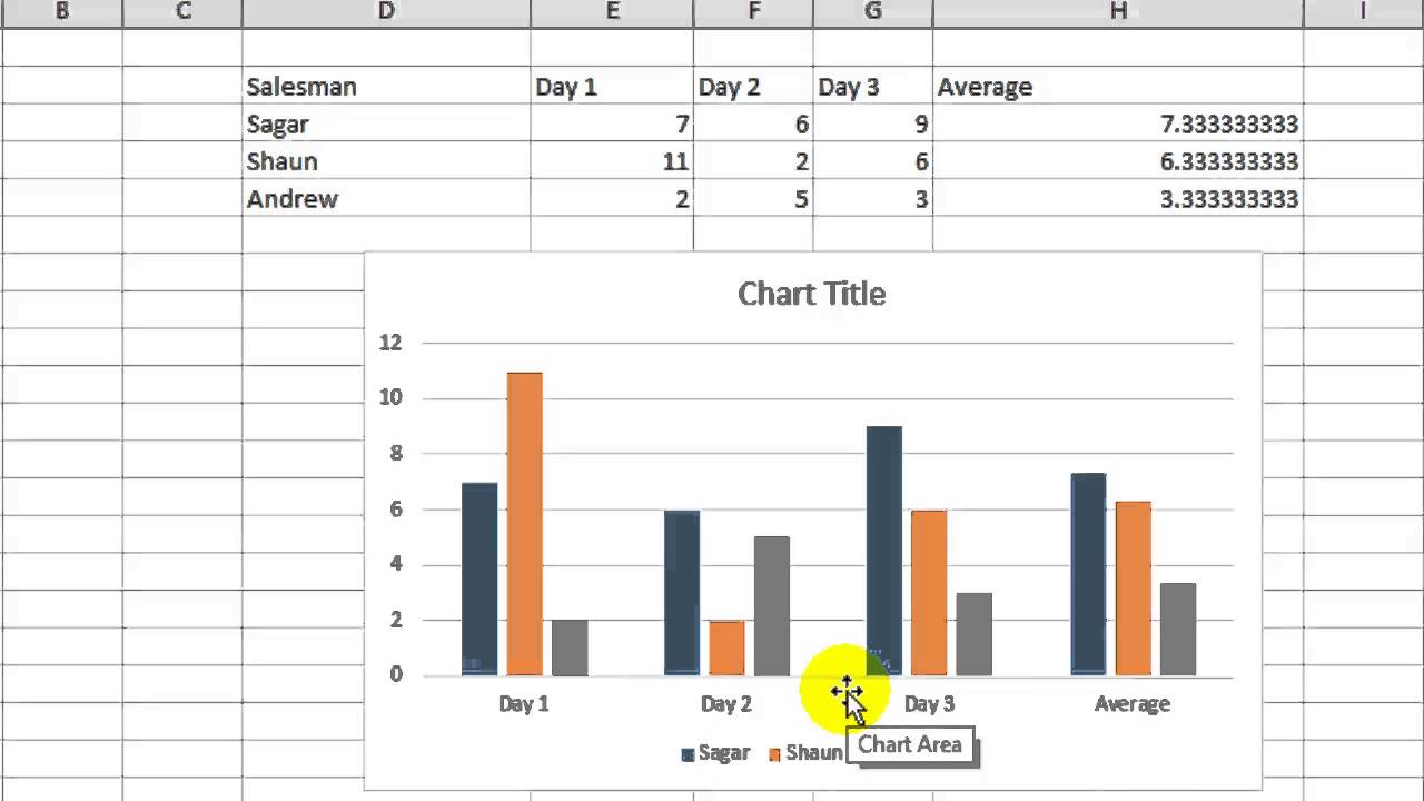
How to use cell values for excel chart labels - How to We want to chart the sales values and use the change values for data labels. Use Cell Values for Chart Data Labels. Select range A1:B6 and click Insert > Insert Column or Bar Chart > Clustered Column. The column chart will appear. We want to add data labels to show the change in value for each product compared to last month.
34 How To Label A Chart In Excel - Label Ideas 2020
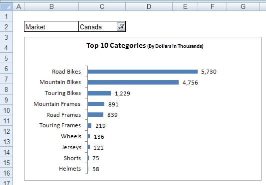
peltiertech.com › text-labels-on-horizontal-axis-in-eText Labels on a Horizontal Bar Chart in Excel - Peltier Tech Dec 21, 2010 · In this tutorial I’ll show how to use a combination bar-column chart, in which the bars show the survey results and the columns provide the text labels for the horizontal axis. The steps are essentially the same in Excel 2007 and in Excel 2003. I’ll show the charts from Excel 2007, and the different dialogs for both where applicable.

add labels to excel chart 218253.image0 - Top Label Maker
› make-labels-with-excel-4157653How to Print Labels from Excel - Lifewire Apr 05, 2022 · Connect the Worksheet to the Labels . Before performing the merge to print address labels from Excel, you must connect the Word document to the worksheet containing your list. The first time you connect to an Excel worksheet from Word, you must enable a setting that allows you to convert files between the two programs.
Formula Friday - Using Formulas To Add Custom Data Labels To Your Excel Chart - How To Excel At ...
How To Create Labels In Excel • ridealert Click yes to merge labels from excel to word. Then click the chart elements, and check data labels, then you can click the arrow to choose an option about the data labels in the sub menu.see screenshot: Source: . Click "labels" on the left side to make the "envelopes and labels" menu appear. Open a data source and merge ...
Excel Custom Chart Labels • My Online Training Hub
Manage sensitivity labels in Office apps - Microsoft Purview ... In Excel, the label applies the watermark text "Confidential". In Outlook, the label doesn't apply any watermark text because watermarks as visual markings are not supported for Outlook. ... Outlook will always use the value you specify for Apply this label by default to documents on the Policy settings for documents page of the label policy ...

Directly Labeling Excel Charts | PolicyViz
› 509290 › how-to-use-cell-valuesHow to Use Cell Values for Excel Chart Labels - How-To Geek Mar 12, 2020 · The values from these cells are now used for the chart data labels. If these cell values change, then the chart labels will automatically update. Link a Chart Title to a Cell Value. In addition to the data labels, we want to link the chart title to a cell value to get something more creative and dynamic.
Excel Custom Chart Labels • My Online Training Hub
› charts › dynamic-chart-dataCreate Dynamic Chart Data Labels with Slicers - Excel Campus Feb 10, 2016 · The next step is to change the data labels so they display the values in the cells that contain our CHOOSE formulas. As I mentioned before, we can use the “Value from Cells” feature in Excel 2013 or 2016 to make this easier. You basically need to select a label series, then press the Value from Cells button in the Format Data Labels menu.

How to sort data with Microsoft Excel 2016 - MATC Information Technology Programs: Degrees ...
How to List and Sort Unique Values and Text in Microsoft Excel Use 1 for ascending order and -1 for descending order. If no value is used, the function assumes 1 by default. Combine Unique Values One more handy addition to the UNIQUE function allows you to combine values. For instance, maybe your list has values in two columns instead of just one as in the screenshot below.

Excel - Sort Labels in a Chart - YouTube
peltiertech.com › prevent-overlapping-data-labelsPrevent Overlapping Data Labels in Excel Charts - Peltier Tech May 24, 2021 · Overlapping Data Labels. Data labels are terribly tedious to apply to slope charts, since these labels have to be positioned to the left of the first point and to the right of the last point of each series. This means the labels have to be tediously selected one by one, even to apply “standard” alignments.

Multiple Series in One Excel Chart - Peltier Tech Blog
How to Fix a Convert to Number Error in Excel - Sheetaki Next, select the values you want to convert into numbers. In this case, we'll select the range C3:C8. ... This guide will show you how to add axis labels to charts in Excel. Creating charts and graphs… Read More. M Microsoft Excel. How To Use SUMPRODUCT Function in Excel. by Deion Menor;
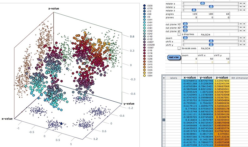
3d scatter plot for MS Excel
IF AND in Excel: nested formula, multiple statements, and more For the formula to work correctly in all the rows, be sure to use absolute references for the boundary cells ($F$1 and $F$2 in our case): =IF (AND (B2>=$F$1, B2<=$F$2), "x", "") By using a similar formula, you can check if a date falls within a specified range. For example, let's flag dates between 10-Sep-2018 and 30-Sep-2018, inclusive.
![Custom Data Labels with Colors and Symbols in Excel Charts - [How To] | Microsoft excel formulas ...](https://i.pinimg.com/originals/e2/41/5e/e2415eb0d7de8ffbc22568267cf3924a.gif)
Custom Data Labels with Colors and Symbols in Excel Charts - [How To] | Microsoft excel formulas ...
How do I make multiple row labels in a PivotTable? In the PivotTable, right-click a value and select Group. In the Grouping box, select Starting at and Ending at checkboxes, and edit the values if needed. Under By, select a time period. For numerical fields, enter a number that specifies the interval for each group. Select OK. How to put row labels next to each other in pivot table?
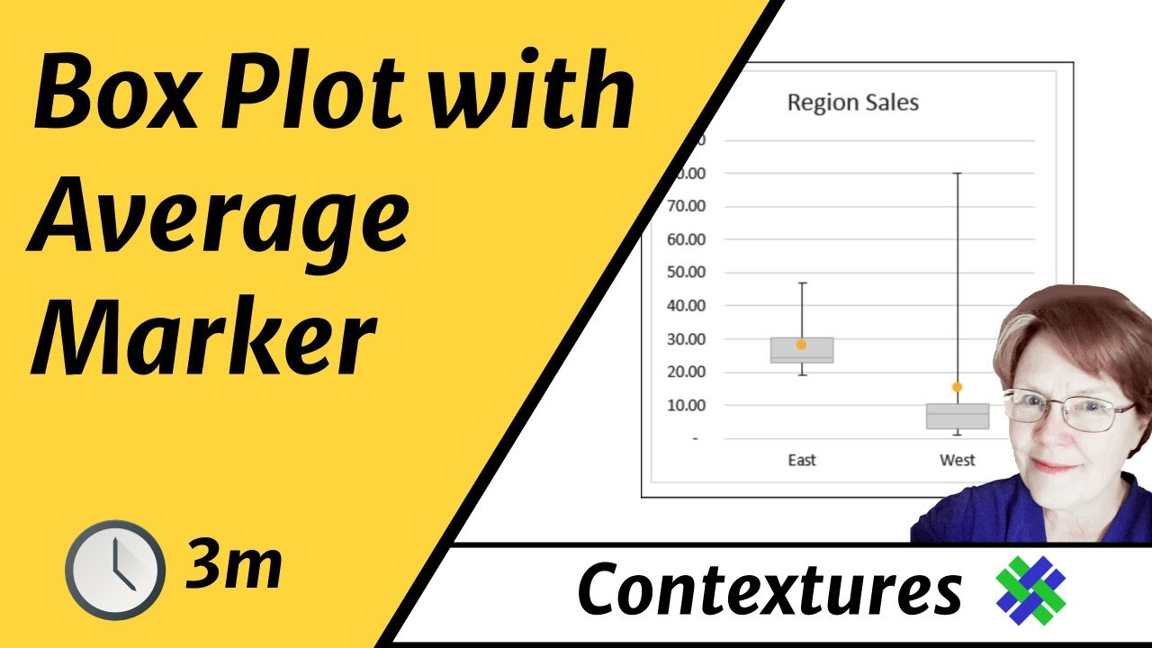
Add Average Marker to Excel Box Plot - Box and Whisker Chart - YouTube
Formatting data labels does not save changes - Microsoft Community Hello, When I remove "values" via format data labels, on a Pivot Chart, when I save the file and reopen it, the data lables re-appear, I believe the changes I make in the formatting should stay in the ... I've tried in Excel as you described and I encountered exactly the same problem. So it is probably a bug which needs to be fixed. I'm going ...
How to change x axis values in Microsoft excel - YouTube
X Axis Labels Below Negative Values - Beat Excel! To do so, double-click on x axis labels. This will open "Format Axis" menu on left side of the screen. Make sure "Format Axis" menu is selected and if not, click on the area marked with dark green. This will open Format Axis menu. Then click on "Labels" as shown below. While in Labels menu, navigate to label position and select "Low".
31 What Is A Category Label In Excel - Labels Database 2020
Custom Chart Data Labels In Excel With Formulas - How To Excel At Excel Follow the steps below to create the custom data labels. Select the chart label you want to change. In the formula-bar hit = (equals), select the cell reference containing your chart label's data. In this case, the first label is in cell E2. Finally, repeat for all your chart laebls.
Post a Comment for "45 labels and values in excel"