42 how to add data labels in excel graph

How to create Custom Data Labels in Excel Charts - Efficiency 365 Create the chart as usual. Add default data labels. Click on each unwanted label (using slow double click) and delete it. Select each item where you want the custom label one at a time. Press F2 to move focus to the Formula editing box. Type the equal to sign. Now click on the cell which contains the appropriate label. How to make a Gantt chart in Excel - Ablebits.com May 23, 2014 · Remove excess white space between the bars. Compacting the task bars will make your Gantt graph look even better. Click any of the orange bars to get them all selected, right click and select Format Data Series.; In the Format Data Series dialog, set Separated to 100% and Gap Width to 0% (or close to 0%).; And here is the result of our efforts - a simple but …

How to Add X and Y Axis Labels in Excel (2 Easy Methods) In short: Select graph > Chart Design > Add Chart Element > Axis Titles > Primary Horizontal. Afterward, if you have followed all steps properly, then the Axis Title option will come under the horizontal line. But to reflect the table data and set the label properly, we have to link the graph with the table.

How to add data labels in excel graph

How to add data labels from different column in an Excel chart? This method will introduce a solution to add all data labels from a different column in an Excel chart at the same time. Please do as follows: 1. Right click the data series in the chart, and select Add Data Labels > Add Data Labels from the context menu to add data labels. 2. How to Add Two Data Labels In Excel Chart? - YouTube In this video tutorial, we are going to learn, how to add multiple data labels in excel pie chart.Our YouTube Channels Travel Volg Channelhttps:// ... › charts › dynamic-chart-dataCreate Dynamic Chart Data Labels with Slicers - Excel Campus Feb 10, 2016 · For now we will just add a cell that contains the index number, and point to the three metrics for each value in the CHOOSE formula. Eventually the slicer will control the index number. Step 5: Setup the Data Labels. The next step is to change the data labels so they display the values in the cells that contain our CHOOSE formulas.

How to add data labels in excel graph. Polar Plot in Excel - Peltier Tech Nov 17, 2014 · Excel has plotted the XY data on secondary axes: the axis labels of both are plainly visible in the left chart below. ... Add labels to the new series; the default Y values are used in the labels (below left). ... Create tables of equal latitude points as would be viewed from above the north pole for 0 to 360 degrees and add as XY graph (smooth ... How to Add, Edit and Rename Data Labels in Excel Charts In this tutorial, you will learn how to add, edit and rename data labels in Microsoft excel graphs.#DataLabels #DataLabel #ExcelChart #ExcelGraph How To Add Data Labels In Excel -* Petitmarche The column chart will appear. For example, this is how we can add labels to one of the data series in our excel chart: Source: . Click the + symbol and add data labels by clicking it as shown below step 3: Click add chart element and select data labels, and then select a location for the data label option. Source: engineerexcel.com › 3-axis-graph-excel3 Axis Graph Excel Method: Add a Third Y-Axis - EngineerExcel By default, Excel adds the y-values of the data series. In this case, these were the scaled values, which wouldn’t have been accurate labels for the axis (they would have corresponded directly to the secondary axis). However, in Excel 2013 and later, you can choose a range for the data labels. For this chart, that is the array of unscaled ...

How to Change Excel Chart Data Labels to Custom Values? - Chandoo.org May 05, 2010 · First add data labels to the chart (Layout Ribbon > Data Labels) Define the new data label values in a bunch of cells, like this: Now, click on any data label. This will select “all” data labels. Now click once again. At this point excel will select only one data label. › documents › excelHow to add data labels from different column in an Excel chart? This method will introduce a solution to add all data labels from a different column in an Excel chart at the same time. Please do as follows: 1. Right click the data series in the chart, and select Add Data Labels > Add Data Labels from the context menu to add data labels. 2. Add a DATA LABEL to ONE POINT on a chart in Excel Click on the chart line to add the data point to. All the data points will be highlighted. Click again on the single point that you want to add a data label to. Right-click and select ' Add data label ' This is the key step! Right-click again on the data point itself (not the label) and select ' Format data label '. How to☝️Create a Pie of Pie Chart in Excel - SpreadsheetDaddy Start off by following the chart creation method as described below. Select your data. Navigate to the Insert menu. In the Chart submenu, click on Insert Pie or Doughnut Chart. Pick the Pie of Pie Chart type. Voila! With those few steps, you have added a Pie of Pie Chart to your worksheet.

Find, label and highlight a certain data point in Excel scatter graph Here's how: Click on the highlighted data point to select it. Click the Chart Elements button. Select the Data Labels box and choose where to position the label. By default, Excel shows one numeric value for the label, y value in our case. To display both x and y values, right-click the label, click Format Data Labels…, select the X Value and ... Excel: How to Create a Bubble Chart with Labels - Statology However, it's tough to know which bubbles represent which players because there are no labels. Step 3: Add Labels. To add labels to the bubble chart, click anywhere on the chart and then click the green plus "+" sign in the top right corner. Then click the arrow next to Data Labels and then click More Options in the dropdown menu: In the ... Edit titles or data labels in a chart - support.microsoft.com On a chart, click one time or two times on the data label that you want to link to a corresponding worksheet cell. The first click selects the data labels for the whole data series, and the second click selects the individual data label. Right-click the data label, and then click Format Data Label or Format Data Labels. › charts › add-data-pointAdd Data Points to Existing Chart – Excel & Google Sheets Start with your Graph. Similar to Excel, create a line graph based on the first two columns (Months & Items Sold) Right click on graph; Select Data Range . 3. Select Add Series. 4. Click box for Select a Data Range. 5. Highlight new column and click OK. Final Graph with Single Data Point

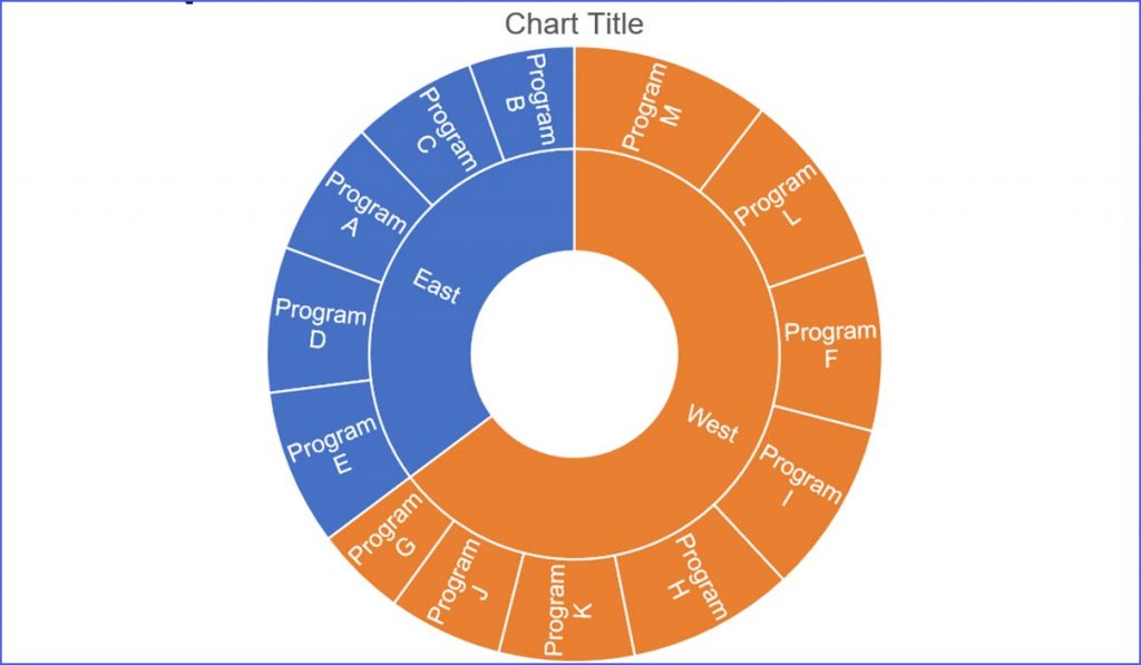
How to Make a Sunburst Chart - ExcelNotes

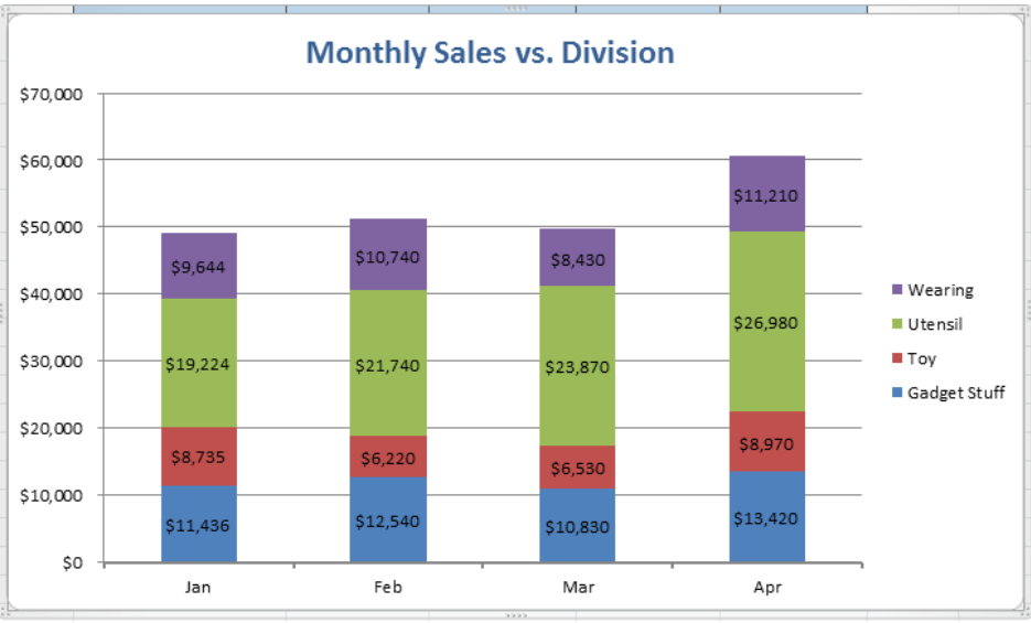
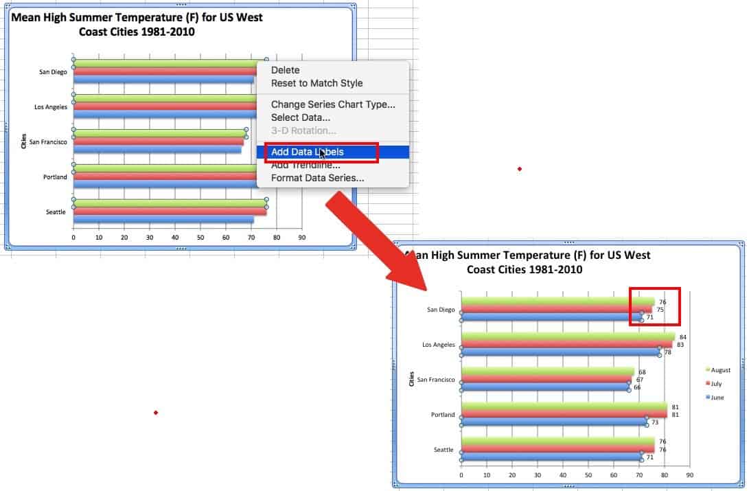
How to Add Total Data Labels to the Excel Stacked Bar Chart Apr 03, 2013 · Step 4: Right click your new line chart and select “Add Data Labels” Step 5: Right click your new data labels and format them so that their label position is “Above”; also make the labels bold and increase the font size. Step 6: Right click the line, select “Format Data Series”; in the Line Color menu, select “No line”

32 What Is A Data Label In Excel - Labels Design Ideas 2020

How to Map Data in Excel (2 Easy Methods) - ExcelDemy Jun 12, 2022 · The data map is one of them. Additionally, it is widely used for visualizing different datasets from various fields. If you are looking for some special tricks to map data in excel, you’ve come to the right place. There are numerous ways to map data in excel. This article will discuss two suitable methods to map data in excel.

How to Add Data Labels in Excel - Excelchat | Excelchat

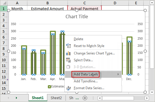
Add or remove data labels in a chart - support.microsoft.com Add data labels to a chart Click the data series or chart. To label one data point, after clicking the series, click that data point. In the upper right corner, next to the chart, click Add Chart Element > Data Labels. To change the location, click the arrow, and choose an option.

How to change date format in axis of chart/Pivotchart in Excel?

3 Axis Graph Excel Method: Add a Third Y-Axis - EngineerExcel Scale the Data for an Excel Graph with 3 Variables. ... Add Data Labels To a Multiple Y-Axis Excel Chart. Axis labels were created by right-clicking on the series and selecting “Add Data Labels”. By default, Excel adds the y-values of the data series. In this case, these were the scaled values, which wouldn’t have been accurate labels for ...

Enable or Disable Excel Data Labels at the click of a button - How To - PakAccountants.com

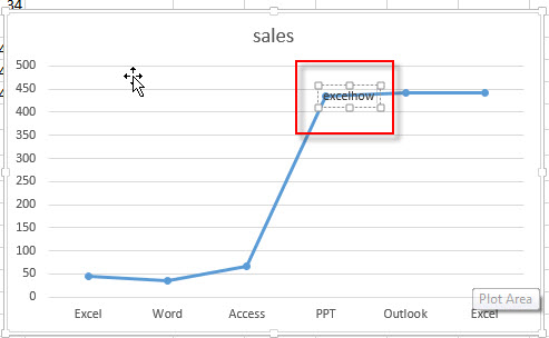
How to add a line in Excel graph: average line, benchmark, etc. Sep 12, 2018 · Right-click the selected data point and pick Add Data Label in the context menu: The label will appear at the end of the line giving more information to your chart viewers: Add a text label for the line. To improve your graph further, you may wish to add a text label to the line to indicate what it actually is. Here are the steps for this set up:

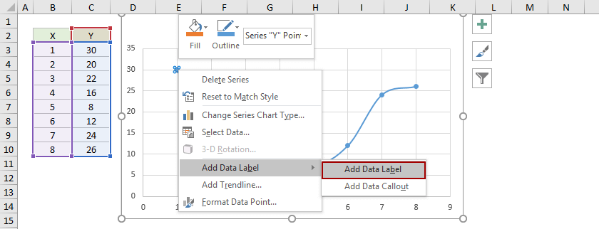
How to add data labels from different column in an Excel chart?

Change the format of data labels in a chart You can add a built-in chart field, such as the series or category name, to the data label. But much more powerful is adding a cell reference with explanatory text or a calculated value. Click the data label, right click it, and then click Insert Data Label Field. If you have selected the entire data series, you won't see this command.

Excel Course: Inserting Graphs

How to add data labels in excel to graph or chart (Step-by-Step) Add data labels to a chart 1. Select a data series or a graph. After picking the series, click the data point you want to label. 2. Click Add Chart Element Chart Elements button > Data Labels in the upper right corner, close to the chart. 3. Click the arrow and select an option to modify the location. 4.

Xyz graf excel | there are several different equations you need in order

Add data labels and callouts to charts in Excel 365 - EasyTweaks.com Step #1: After generating the chart in Excel, right-click anywhere within the chart and select Add labels . Note that you can also select the very handy option of Adding data Callouts.

Need help making labels on a graph with format code : excel

Change the format of data labels in a chart To get there, after adding your data labels, select the data label to format, and then click Chart Elements > Data Labels > More Options. To go to the appropriate area, click one of the four icons ( Fill & Line, Effects, Size & Properties ( Layout & Properties in Outlook or Word), or Label Options) shown here.

How to Make a Data Comparison Graph in Excel 2016 Spreadsheet

Excel Charts: Creating Custom Data Labels - YouTube In this video I'll show you how to add data labels to a chart in Excel and then change the range that the data labels are linked to. This video covers both W...

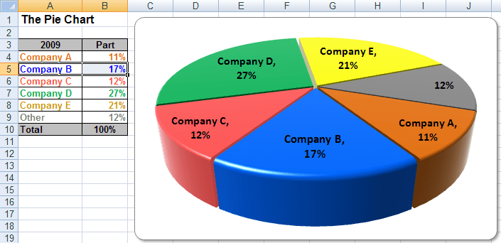
Excel 3-D Pie Charts

How to Select Data for Graphs in Excel - Sheetaki Select the blank graph and navigate to the Chart Design tab. Click on the Select Data option. In the Select Data Source dialog box, select the Chart data range text box and type in your range. You may also use your cursor to select the range much faster. Click on the OK button to apply the new data source to your graph.

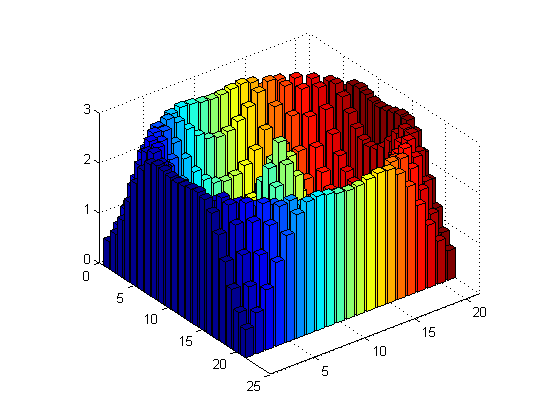
More advanced plotting features

how to add data labels into Excel graphs - storytelling with data You can download the corresponding Excel file to follow along with these steps: Right-click on a point and choose Add Data Label. You can choose any point to add a label—I'm strategically choosing the endpoint because that's where a label would best align with my design. Excel defaults to labeling the numeric value, as shown below.

charts - Excel, giving data labels to only the top/bottom X% values - Stack Overflow

› excel › how-to-add-total-dataHow to Add Total Data Labels to the Excel Stacked Bar Chart Apr 03, 2013 · Step 4: Right click your new line chart and select “Add Data Labels” Step 5: Right click your new data labels and format them so that their label position is “Above”; also make the labels bold and increase the font size. Step 6: Right click the line, select “Format Data Series”; in the Line Color menu, select “No line” Step 7 ...

How to Make a Bar Chart in Excel | Smartsheet

How to Add Data Labels in Excel - Excelchat | Excelchat After inserting a chart in Excel 2010 and earlier versions we need to do the followings to add data labels to the chart; Click inside the chart area to display the Chart Tools. Figure 2. Chart Tools Click on Layout tab of the Chart Tools. In Labels group, click on Data Labels and select the position to add labels to the chart. Figure 3.

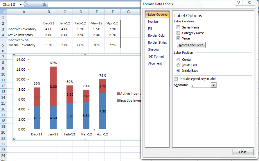
How-to Put Percentage Labels on Top of a Stacked Column Chart - Excel Dashboard Templates

Add Data Points to Existing Chart – Excel & Google Sheets Start with your Graph. Similar to Excel, create a line graph based on the first two columns (Months & Items Sold) Right click on graph; Select Data Range . 3. Select Add Series. 4. Click box for Select a Data Range. 5. Highlight new column and …

Excel Chart Elements: Parts of Charts in Excel | ExcelDemy

Custom Chart Data Labels In Excel With Formulas - How To Excel At Excel Follow the steps below to create the custom data labels. Select the chart label you want to change. In the formula-bar hit = (equals), select the cell reference containing your chart label's data. In this case, the first label is in cell E2. Finally, repeat for all your chart laebls.

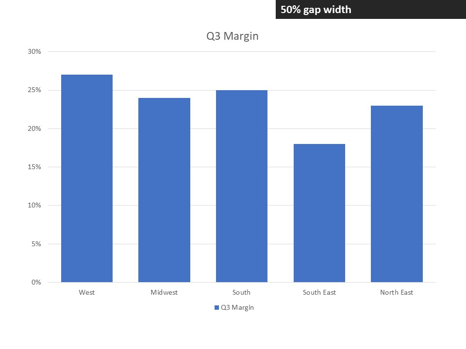
7 Steps to make a professional looking column graph in Excel or PowerPoint | Think Outside The Slide

› 2018/09/12 › add-line-excel-graphHow to add a line in Excel graph (average line, benchmark ... Sep 12, 2018 · Right-click the selected data point and pick Add Data Label in the context menu: The label will appear at the end of the line giving more information to your chart viewers: Add a text label for the line. To improve your graph further, you may wish to add a text label to the line to indicate what it actually is. Here are the steps for this set up:

Share :